Python, Numpy, Pandas and Matplotlib notes
Table of Contents
- Table of Contents
Java vs Python
Unlike in Java, in Python, we do not use the semicolon ;, nor curly brackets {} to denote code blocks. Instead, a line break denotes the end of a statement and indentation is used to denote code blocks. Take the following Java method:
public void foo(boolean bar) {
    if (bar) {
        System.out.println("Hello world");
    } else {
        System.out.println("42");
    }
}
In Python, this would be written as:
def foo(bar):
    if bar:
        print("Hello World")
    else:
        print("42")
Python program files on Unix
- Python code is usually stored in text files with the file ending “.py”:
myprogram.py - Every line in a Python program file is assumed to be a Python statement, or part thereof.
- The only exception is comment lines, which start with the character
#(optionally preceded by an arbitrary number of white-space characters, i.e., tabs or spaces). Comment lines are ignored by the Python interpreter.
- The only exception is comment lines, which start with the character
- To run our Python program from the command line, use:
$ python myprogram.py
- On UNIX systems it is common to define the path to the interpreter on the first line of the program (note that this is a comment line as far as the Python interpreter is concerned):
#!/usr/bin/env python
- If we do, and if we additionally set the file script to be executable, we can run the program like this:
$ myprogram.py
Modules
- Most of the functionality in Python is provided by modules. The Python Standard Library is a large collection of modules that provides cross-platform implementations of common facilities such as access to the operating system, file I/O, string management, network communication, and much more.
- To use a module in a Python program it first has to be imported. A module can be imported using the import statement. To import the module math, which contains many standard mathematical functions, we can do:
import math
- This includes the whole module and makes it available for use later in the program. For example, we can write the following program using the math module:
import math

math.cos(2 * math.pi)
- Alternatively, we can choose to import all symbols (functions and variables) in a module to the current namespace (so that we don’t need to use the prefix “math.” every time we use something from the math module):
from math import *

cos(2 * pi)
- This pattern can be very convenient, but in large programs that include many modules it is often a good idea to keep the symbols from each module in their own namespaces, by using the import math pattern. This would eliminate potentially confusing problems with name space collisions.
- As a third alternative, we can choose to import only a few selected symbols from a module by explicitly listing which ones we want to import instead of using the wildcard character *:
from math import cos, pi

cos(2 * pi)
- Once a module is imported, we can list the symbols it provides using the dir function:
import math
dir(math)
Which returns: [‘__doc__’, ‘__loader__’, ‘__name__’, ‘__package__’, ‘__spec__’, ‘acos’, ‘acosh’, ‘asin’…]
- And using the function help we can get a description of each function (almost .. not all functions have docstrings, as they are technically called, but the vast majority of functions are documented this way).
help(math.log)
Help on built-in function log in module math:

log(...)
    log(x, [base=math.e])
    Return the logarithm of x to the given base.

    If the base not specified, returns the natural logarithm (base e) of x.
- We can also use the help function directly on modules i.e.
help(math) -
Some very useful modules form the Python standard library are os, sys, math, shutil, re, subprocess, multiprocessing, threading.
- We can (and should) create our own modules that abstract/refactor functionalities into a
.pyfile (module).- While functions and classes (within a file) are examples of tools for low-level modular programming. Python modules are a higher-level modular programming construct, where we can collect related variables, functions and classes in a module.
- Like the Python libraries, you import your own modules with the
importstatement
- Consider the following example: the file
mymodule.pycontains simple example implementations of a variable, function and a class:
%%file mymodule.py
"""
Example of a Python module. Contains a variable called my_variable,
a function called my_function, and a class called MyClass.
"""
my_variable = 0
def my_function():
"""
Example function
"""
return my_variable
class MyClass:
"""
Example class.
"""
def __init__(self):
self.variable = my_variable
def set_variable(self, new_value):
"""
Set self.variable to a new value
"""
self.variable = new_value
def get_variable(self):
return self.variable
- We can import the module mymodule into other program with:
%load_ext autoreload
%autoreload 2 # This makes sure all modules are reloaded every time before executing the Python code typed.

import mymodule
Variables and types
- Variable names in Python can contain alphanumerical characters a-z, A-Z, 0-9 and some special characters such as _. Normal variable names must start with a letter.
- By convention, variable names start with a lower-case letter, and Class names start with a capital letter. Another convention is to use the lower dash _ to separate words, instead of camelcase. E.g. instead of myVariable, we tend to write my_variable. For further code style guidlines, you can check out Google’s style guides for python: http://google.github.io/styleguide/pyguide.html
- In addition, there are a number of Python keywords that cannot be used as variable names. These keywords are:
- and, as, assert, break, class, continue, def, del, elif, else, except, exec, finally, for, from, global, if, import, in, is, lambda, not, or, pass, print, raise, return, try, while, with, yield
- The assignment operator in Python is
=. Like Javascript, python is a dynamically typed language, so we do not need to specify the type of a variable when we create one. The type is derived from the value it was assigned.
Assigning a value to a new variable creates the variable:
# variable assignments
x = 1.0
my_variable = 12.2

type(x) # check the type (returns "int")
- If we assign a new value to a variable, its type can change.
x =[1,2,3,4,5]
type(x) # should return "list"
- If we try to use a variable that has not yet been defined we get a NameError:
y
returns:
---------------------------------------------------------------------------
NameError                                 Traceback (most recent call last)
<ipython-input-13-9063a9f0e032> in <module>
----> 1 y

NameError: name 'y' is not defined
- Python has four primitive or fundamental data types, namely, integers, floats, booleans and strings. Other types such as complex numbers are also supported:
# complex numbers: note the use of `j` to specify the imaginary part
type(1.0 - 1.0j) # should return "complex"
Type casting
Examples of type casting in Python are shown below.
x = 1.5
print(x, type(x))
x = int(x)
print(x, type(x))
z = complex(x)
print(z, type(z))
x = float(z)
---------------------------------------------------------------------------
TypeError                                 Traceback (most recent call last)
<ipython-input-24-19c840f40bd8> in <module>
----> 1 x = float(z)

TypeError: can't convert complex to float
- Complex variables cannot be cast to floats or integers. We need to use
z.realorz.imagto extract the part of the complex number we want:
y = bool(z.real)
print(z.real, " -> ", y, type(y))
y = bool(z.imag)
print(z.imag, " -> ", y, type(y))
1.0  ->  True <class 'bool'>
0.0  ->  False <class 'bool'>
Operators and comparisons
- Arithmetic operators +, -, *, /, // (integer division), % (modulo), ** power
- The boolean operators are spelled out as words: and, not, or.
True and False
False
not False
True
True or False
True
- Comparison operators >, <, >= (greater or equal), <= (less or equal), == (equality), is (identical as if same memory address)
# equality
[1,2] == [1,2]
True
# objects identical (same memory adress)?
o1 = [1,2]
o2 = [1,2]

o1 is o2
False
Compound types
Strings
- Strings are the variable type that is used for storing text.
s = "Hello world"
type(s)
str.capitalize('abcd') #'Abcd'
# length of the string: the number of characters including spaces
len(s)
# replace a substring in a string with something else
s2 = s.replace("world", "test")
print(s2)
Hello test
- We can index a character in a string using []:
s[0]
H
- Unlike MATLAB, indexing start at 0!
-
We can extract a part of a string using the syntax [start:stop], which extracts characters between index start and stop, including the start element and excluding the stop element: [start, stop).
- If we do not define start or stop in [start:stop], e.g. [:stop], start will default to 0 and end to the end of the string.
s[:5]
Hello
s[6:]
world
s[:]
Hello world
- We can also define the step size using the syntax [start:end:step] (the default value for step is 1, as we saw above). This technique is called slicing.
s[::1]
Hello world
s[::2]
Hlowrd
String formatting
print("str1", "str2", "str3")  # The print statement concatenates strings with a space

print("str1", 1.0, False, -1j)  # The print statements converts all arguments to strings

print("str1" + "str2" + "str3") # strings added with + are concatenated without space
print("value = %f" % 1.0) # we can use C-style string formatting
value = 1.000000
s2 = "value1 = %.2f. value2 = %d" % (3.1415, 1.5) # returns: value1 = 3.14. value2 = 1

# alternative, more intuitive way of formatting a string
s3 = 'value1 = {0}, value2 = {1}'.format(3.1415, 1.5) # returns: value1 = 3.1415, value2 = 1.5
Lists
- Lists are very similar to strings, except that each element can be of any type.
- The syntax for creating lists in Python is [value_1,value_2, … ,value_n]:
l = [1,2,3,4]
print(type(l))
print(l)
<class 'list'>
[1, 2, 3, 4]
- We can use the same slicing techniques to manipulate lists as we could use on strings:
print(l)
print(l[1:3])
print(l[::2])
[1, 2, 3, 4]
[2, 3]
[1, 3]
- Elements in a list do not all have to be of the same type. However, to avoid errors, it is advised to store only values of one type in a list:
- Python lists can be inhomogeneous and arbitrarily nested:
nested_list = [1, [2, [3, [4, [5]]]]]
- Lists play a very important role in Python, and are used in loops and other flow control structures (discussed below). There are a number of convenient functions for generating lists of various types, for example the range function:
start = 10
stop = 30
step = 2
range(start, stop, step) # range(10, 30, 2)
# in python 3 range generates an iterator, which can be converted to a list using 'list(...)'.
list(range(start, stop, step))
[10, 12, 14, 16, 18, 20, 22, 24, 26, 28]
list(range(-10, 10)) # no step means step = 1
[-10, -9, -8, -7, -6, -5, -4, -3, -2, -1, 0, 1, 2, 3, 4, 5, 6, 7, 8, 9]
- convert a string to a list by type casting:
s = 'Hello world'
s2 = list(s) #= ['H', 'e', 'l', 'l', 'o', ' ', 'w', 'o', 'r', 'l', 'd']
- sorting lists, uppercase and lowercase characters are sorted separately
s2.sort()
print(s2)
[' ', 'H', 'd', 'e', 'l', 'l', 'l', 'o', 'o', 'r', 'w']
Adding, inserting, modifying, and removing elements from lists
- create a new empty list with
l = [] - add an elements using
append
l.append("A")
l.append("d")
l.append("d")
print(l)
['A', 'd', 'd']
- We can modify lists by assigning new values to elements in the list. In technical jargon, lists are mutable.
l[1] = "p"
l[2] = "p"
print(l)
['A', 'p', 'p']
- Insert an element at an specific index using insert
l.insert(0, "i")
l.insert(1, "n")
l.insert(2, "s")
l.insert(3, "e")
l.insert(4, "r")
l.insert(5, "t")
- Remove first element with specific value using ‘remove’:
l.remove("A") - Remove an element at a specific location using del:
del l[7] - See help(list) for more details, or read the online documentation
Tuples
- Tuples are like lists, except that they cannot be modified once created, that is they are immutable.
- In Python, tuples are created using the syntax (…, …, …):
point = (10, 20)
print(point, type(point))
(10, 20) <class 'tuple'>
- We can unpack a tuple by assigning it to comma-separated variables:
x, y = point
print("x =", x)
print("y =", y)

x = 10
y = 20
- If we try to assign a new value to an element in a tuple we get an error:
point[0] = 20
---------------------------------------------------------------------------
TypeError                                 Traceback (most recent call last)
<ipython-input-70-9734b1daa940> in <module>
----> 1 point[0] = 20

TypeError: 'tuple' object does not support item assignment
Dictionaries
- Dictionaries are also like Java objects. The values are connected to keys of the dictionary. The keys can be used to retrieve values from a dictionary. The syntax for dictionaries is {key1 : value1, …}:
values = {
"key1" : 1.0,
"key2" : 2,
"key3" : [1,2,3]
}
print(type(values))
print(values)
<class 'dict'>
{'key1': 1.0, 'key2': 2, 'key3': [1, 2, 3]}
- Retrieve a value by using the key
values["key1"]
1.0
- You can reassign the values corresponding to a key
values["key1"] = "A"
values["key2"] = "B"
values["key4"] = "D" # Assigning a value to an unknown key results in the creation of that key

print("key1 = ", values["key1"])
print("key2 = ", values["key2"])
print("key3 = ", values["key3"])
print("key4 = ", values["key4"])
key1 =  A
key2 =  B
key3 =  [1, 2, 3]
key4 =  D
Control Flow
Conditional blocks
- The Python syntax for conditional execution of code use the keywords if, elif (else if), else
- Program blocks are defined by their indentation level.
statement1 = False
statement2 = False

if statement1:
    print("statement1 is True")

elif statement2:
    print("statement2 is True")

else:
    print("statement1 and statement2 are False")
Loops
- In Python, loops can be programmed in a number of different ways. The most common is the for loop, which is used together with iterable objects with in, such as lists. The basic syntax is: for loops:
for x in [1,2,3]:
    print(x)
- The for loop iterates over the elements of the supplied list, and executes the containing block once for each element.
- Any kind of list can be used in the for loop:
for x in range(4): # by default range start at 0
    print(x)
- To iterate over key-value pairs of a dictionary one can also jus use in:
values = {
"key1" : 1.0,
"key2" : 2,
"key3" : [1,2,3]
}
for key, value in values.items():
print(key + " = " + str(value))
- Sometimes it is useful to have access to the indices of the values when iterating. We can use the enumerate function for this:
for index, x in enumerate(range(-3,3)):
    print(index, x)
- A convenient and compact way to initialize lists can be done with for loops:
l1 = [x**2 for x in range(0,5)] # yikes
print(l1)
[0, 1, 4, 9, 16]
While loops
- It’s your job to update the conditional variable such that to not end up with an infinite loop
i = 0

while i < 5:
    print(i)
    i = i + 1
Functions
- A function (method in Java) in Python is defined using the keyword
def, followed by a function name, a signature (lists the parameters) within parentheses(), and a colon:. The following code, with one additional level of indentation, is the function body.
def func0():
    print("func0 is called")

func0()
func0 is called
- Optionally, but highly recommended, we can define a so called “docstring”, which is a description of the function’s purpose and behaivor. The docstring should follow directly after the function definition, before the code in the function body.
def func1(s):
    """
    Print a string 's' and tell how many characters it has
    """
    print(s + " has " + str(len(s)) + " characters")

help(func1)
Help on function func1 in module __main__:
func1(s)
    Print a string 's' and tell how many characters it has
- Functions that return a value use the return keyword (see that the fuction keywords remain the same):
def square(x):
    """
    Return the square of x.
    """
    return x ** 2
- We can return multiple values from a function using tuples (see above):
def powers(x):
    """
    Return a few powers of x.
    """
    return x ** 2, x ** 3, x ** 4
print(powers(3))
(9, 27, 81)
x2, x3, x4 = powers(3)
print(x3)
27
- In a definition of a function, we can give default values to the arguments the function takes:
- If we don’t provide a value of the debug argument when calling the the function myfunc it defaults to the value provided in the function definition
def myfunc(x, p=2, debug=False):
    if debug:
        print("evaluating myfunc for x = " + str(x) + " using exponent p = " + str(p))
    return x**p
- If we explicitly list the name of the arguments in the function calls, they do not need to come in the same order as in the function definition. This is called keyword arguments, and is often very useful in functions that takes a lot of optional arguments:
myfunc(p=3, debug=True, x=7) - In Python we can also create unnamed functions, using the lambda keyword:
f1 = lambda x: x**2
# is equivalent to
def f2(x):
    return x**2
- This technique is useful for example when we want to pass a simple function as an argument to another function, like this:
# map is a built-in python function
map(lambda x: x**2, range(-3,4))

# in python 3 we can use `list(...)` to convert the iterator to an explicit list
list(map(lambda x: x**2, range(-3,4)))
[9, 4, 1, 0, 1, 4, 9]
Classes
- A class is a structure for representing an object and the operations that can be performed on the object.
- In Python a class can contain attributes (variables) and methods (functions).
- A class is defined almost like a function, but using the class keyword, and the class definition usually contains a number of class method definitions (a function in a class).
- Each class method should have an argument
selfas it first argument. This object is a self-reference. (likethisin java, but turns out python requires you to explicitly pass it as first argument) - Some class method names have special meaning, for example:
- __init__: The name of the method that is invoked when the object is first created (like a constructor in java)
- __str__ : A method that is invoked when a simple string representation of the class is needed, as for example when printed. (toString() in java)
- There are many more
- Each class method should have an argument
class Point:
    """
    Simple class for representing a point in a Cartesian coordinate system.
    """

    def __init__(self, x, y):
        """
        Create a new Point at x, y.
        """
        self.x = x
        self.y = y

    def translate(self, dx, dy):
        """
        Translate the point by dx and dy in the x and y direction.
        """
        self.x += dx
        self.y += dy

    def __str__(self):
        return("Point at [%f, %f]" % (self.x, self.y))
- To create a new instance of a class the first argument (the self reference) is skipped
p1 = Point(0, 0) # this will invoke the __init__ method in the Point class
print(p1)         # this will invoke the __str__ method
Point at [0.000000, 0.000000]
- To invoke a class method in the class instance p is like in java or javascript:
print(p1)
p1.translate(0.25, 1.5)
print(p1)
Point at [0.000000, 0.000000]
Point at [0.250000, 1.500000]
- Note that calling class methods can modify the state of that particular class instance, but does not effect other class instances or any global variables. That is one of the nice things about object-oriented design:
- code such as functions and related variables are grouped in separate and independent entities.
Exceptions
- In Python errors are managed with a special language construct called “Exceptions”. When errors occur exceptions can be raised, which interrupts the normal program flow and fallback to somewhere else in the code where the closest try-except statement is defined.
- To generate an exception we can use the
raisestatement, which takes an argument that must be an instance of the class BaseException or a class derived from it.
raise Exception("description of the error")
---------------------------------------------------------------------------
Exception                                 Traceback (most recent call last)
<ipython-input-105-c32f93e4dfa0> in <module>
----> 1 raise Exception("description of the error")

Exception: description of the error
- A typical use of exceptions is to abort functions when some error condition occurs, for example:
def my_function(arguments):

    if not verify(arguments):
        raise Exception("Invalid arguments")

    # rest of the code goes here
Numpy (Arrays)
import numpy as np
- In machine learning we are dealing with massive amounts of data. This data is most often organised in tables (like for example in spreadsheets). When all data elements in a table are of the same datatype (like an integer or a floating point number) the table can be represented with a homogeneous array.
- Languages that are optimally suited for programming with data (like NumPy) are therefore equipped with array data types as an integral part of the language. An array is a data type to store lists of values. We can also create arrays of arrays, resulting in multi-dimensional arrays. NumPy provides tools to work with these multi-dimensional arrays in the form of the
ndarrayclass.
Making a numpy array using Python lists
list1 = [1, 2, 3, 4]
array1 = np.array(list1) # The type of array1 is "numpy.ndarray": an n-dimensional array
print(array1)
[1 2 3 4]
- 2 dimension array:
# Declare an extra list.
list2 = [11, 22, 33, 44]
# Combine the lists into a 2-dimensional list.
lists = [list1, list2]
# make a 2-dimensional NumPy array
array2 = np.array(lists)
print(array2)
[[ 1  2  3  4]
 [11 22 33 44]]
Dimensions, rank, shape, reshape and type
- The number of dimensions is what we call “rank” in linear algebra.
- An array of plain integers has just 1 dimension
- An array of arrays containing plain integers has 2 dimensions
- The “shape” of a numpy array is a tuple of integers giving the size of the array along each dimension:
- When it’s a 1 dimensional array, you get
(len(your_array),) - When it’s n-dimensional (and bigger than 1) you do get (k,l) for 2D, (k,l,m) for 3D etc. with k, l, m n being the size of the array for each dimension
- When it’s a 1 dimensional array, you get
import numpy as np

a = np.array([1, 2, 3])   # Create a rank 1 array
print(type(a))            # Prints "<class 'numpy.ndarray'>"
print(a.shape)            # Prints "(3,)"
print(a[0], a[1], a[2])   # Prints "1 2 3"
a[0] = 5                  # Change an element of the array
print(a)                  # Prints "[5, 2, 3]"

b = np.array([[1,2,3],[4,5,6]])    # Create a rank 2 array
print(b.shape)                     # Prints "(2, 3)"
print(b[0, 0], b[0, 1], b[1, 0])   # Prints "1 2 4"
- See how
shapeandprintare consistent with matlab and linear algebra where the size of a matrix is expressed as rows x columns (m x n).
array3 = np.array([[1, 2, 3, 4], [8, 9, 10, 11]])
#array3
print(array3.shape)
print(array3)
(2, 4)
[[ 1  2  3  4]
 [ 8  9 10 11]]
- In most situations the lack of a second dimension is not a problem. If it does turn into a problem (e.g. when you are trying to take a transpose of this vector) you can just call the reshape function on the array to generate a new view:
# Do note the double brackets, as the size is added as a tuple: (rows, columns)
array1 = array1.reshape((4,1))
array1.shape
(4, 1)
- More reshape:
array8 = np.arange(40)
print(array8)

array8 = array8.reshape((8, 5))
print(array8)
[ 0  1  2  3  4  5  6  7  8  9 10 11 12 13 14 15 16 17 18 19 20 21 22 23 24 25 26 27 28 29 30 31 32 33 34 35 36 37 38 39]
[[ 0  1  2  3  4]
 [ 5  6  7  8  9]
 [10 11 12 13 14]
 [15 16 17 18 19]
 [20 21 22 23 24]
 [25 26 27 28 29]
 [30 31 32 33 34]
 [35 36 37 38 39]]
- For the above examples, we happen to know what we stored in our array, but in some cases we are not aware (like when we imported lots of data). To find out, you can call dtype:
array2.dtype
dtype('int32')
Matlab-like array creation
- Numpy also provides many functions to create arrays:
import numpy as np

a = np.zeros((2,2))   # Create an array of all zeros
print(a)              # Prints "[[ 0.  0.]
                      #          [ 0.  0.]]"

b = np.ones((1,2))    # Create an array of all ones
print(b)              # Prints "[[ 1.  1.]]"

c = np.full((2,2), 7)  # Create a constant array
print(c)               # Prints "[[ 7.  7.]
                       #          [ 7.  7.]]"

d = np.eye(2)         # Create a 2x2 identity matrix
print(d)              # Prints "[[ 1.  0.]
                      #          [ 0.  1.]]"

e = np.random.random((2,2))  # Create an array filled with random values
print(e)                     # Might print "[[ 0.91940167  0.08143941]
                             #               [ 0.68744134  0.87236687]]"

# The empty array (makes an array but doesn't do any initialisation)
print("Ex1: ", np.empty(5))

# Array of 5 integer incrementing numbers
print("Ex4: ", np.arange(5))

# Start at 5, stop at 20, do it in steps of 2
print("Ex5: ", np.arange(5, 20, 2))
Mathematical operations
# Element-wise multiplication
array3 * array3

# Element-wise subtraction
array3 - 5

# Division
1 / array3

# Raising to a power
array3 ** 3

# If you want to transpose a matrix you can do this in two ways:
print(np.transpose(array8))
# Or
print(array8.T)
- The nice thing about NumPy arrays is that it allows you to manipulate the data in arrays without writing explicit loops. For instance look at the addition of all elements in an array:
# Array of random numbers
a = np.random.rand(65536)

#calculate the sum of the elements in array
def loopsum(a):
    sum = 0
    for i in range(len(a)):
        sum += a[i]
    return sum

%timeit loopsum(a)
%timeit np.sum(a)
24.4 ms ± 710 µs per loop (mean ± std. dev. of 7 runs, 10 loops each)
71.4 µs ± 2.65 µs per loop (mean ± std. dev. of 7 runs, 10000 loops each)
- You can see that the numpy loop is about 350 times faster than the explicit loop version. So be aware in this course to use built-in NumPy tools to manipulate and calculate with arrays. Some built-in functions of NumPy can be found here.
Indexing Arrays
- NumPy array allows an additional indexing method
list3 = [[1, 2, 3], [4, 5, 6]]
array5 = np.array(list3)

# Watch the brackets closely.
print("List: ", list3[1][2])
# Array can use two different approaches
print("Array ", array5[1, 2])
print("Array ", array5[1][2]
List:  6
Array  6
Array  6
Slicing arrays
- Sometimes you do not want the full array, but just parts of it, we can use array slicing for this:
# Show original array
print(array5)

# We want the element from the second row and third column:
print(array5[1:2,2:3])
[[1 2 3]
 [4 5 6]]
[[6]]
# We can also use it to set the value of multiple entries:
array4 = np.arange(0, 10)
array4[2:5] = 13
print(array4)
[ 0 1 13 13 13 5 6 7 8 9]
-
One important thing to note is that a slice is just another view of the underlying data buffer. If you change data in the slice, you are actually changing the data in the underlying data buffer and thus in the orginal array.
-
2D array slicing:
array6 = np.array([[2, 4, 6], [8, 10, 12], [14, 16, 18]])
print(array6)

# let's say you only want just the upper right square of 2x2 of the above matrix
# reminder: when indexing with array[start:stop]
# the element at start is *included*, while the elemnt at stop is *excluded*

array6[:2, 1:]
[[ 2  4  6]
 [ 8 10 12]
 [14 16 18]]

array([[ 4,  6],
       [10, 12]])
- Fancy Indexing:
# Sometimes you don't want to retrieve every row, but perhaps skip a few entries. This is easily possible in Python. Let us assume we only want the 2nd, 3rd, 5th, and 7th row in the following example.

# Below we use a list comprehension (which you should have seen in Introduction to Programming as well)
# To generate an array with 10 rows, and each column goes from 0 to 10.
array7 = np.array([[j for i in range(10)] for j in range(10)])
print(array7)

# As we start at index 0, we actually want the following rows [1, 2, 4, 6].
# Also note the double brackets below.

print("With fancy indexing:")
print(array7[[1, 2, 4, 6]])
[[0 0 0 0 0 0 0 0 0 0]
 [1 1 1 1 1 1 1 1 1 1]
 [2 2 2 2 2 2 2 2 2 2]
 [3 3 3 3 3 3 3 3 3 3]
 [4 4 4 4 4 4 4 4 4 4]
 [5 5 5 5 5 5 5 5 5 5]
 [6 6 6 6 6 6 6 6 6 6]
 [7 7 7 7 7 7 7 7 7 7]
 [8 8 8 8 8 8 8 8 8 8]
 [9 9 9 9 9 9 9 9 9 9]]
With fancy indexing:
[[1 1 1 1 1 1 1 1 1 1]
 [2 2 2 2 2 2 2 2 2 2]
 [4 4 4 4 4 4 4 4 4 4]
 [6 6 6 6 6 6 6 6 6 6]]
- You can do the above even in any order you wish.
array7[[6, 2, 4, 1]]
array([[6, 6, 6, 6, 6, 6, 6, 6, 6, 6],
       [2, 2, 2, 2, 2, 2, 2, 2, 2, 2],
       [4, 4, 4, 4, 4, 4, 4, 4, 4, 4],
       [1, 1, 1, 1, 1, 1, 1, 1, 1, 1]])
Array Processing
- We can also apply functions on arrays to retrieve specific information from them, or to process the information that is contained.
Where
- When you want to find the location of elements in an array, you can use np.where. This function takes in a condition and returns the indices of the array where the condition is true.
# A simple np.where example:
A = np.array([1, 2, 3, 4])
indices = np.where(A < 3)
print(indices)
print(A[indices])
(array([0, 1], dtype=int64),)
[1 2]
Boolean array
- As shown before, we can apply a boolean operator on an array, which will return an array with boolean values:
a = np.arange(9).reshape(3, 3)
bool_arr = a < 4
print(bool_arr)
[[ True  True  True]
 [ True False False]
 [False False False]]
Any
- Now, what if we want to return each row where any of the elements is true, we can do that with any in combination with where:
# Return the indices of the rows where any column (axis=1) is true
indices = np.where(bool_arr.any(axis=1))
bool_arr[indices]
# You can see that the last row is excluded as this row doesn't contain any True values
array([[ True,  True,  True],
       [ True, False, False]])
All
- And what if we want all elements in the row to be true? We can use all:
# If all values are true, return true (else false)
indices = np.where(bool_arr.all(axis=1))
bool_arr[indices]
# You can see that only the first row is included as this row is the only one to contain only True values
array([[ True, True, True]])
Unique
# Sometimes you just want to know all the unique values in a numpy array
# Luckily that function was already implemented for you
letters = ['A', 'B', 'C', 'D', 'D', 'A', 'E', 'F', 'G', 'H', 'Z']
np.unique(letters)
array(['A', 'B', 'C', 'D', 'E', 'F', 'G', 'H', 'Z'], dtype='<U1')
In
# We can also easily check whether a big array exists,
# if it exists within a 1D vector.
np.in1d(['X', 'C', 'M', 'Z'], letters)
array([False, True, False, True])
Exercises
- In all exercises below you are not allowed to use a loop.
# Given two arrays A and B each of the same size calculate their sum (elementwise) and their product (elementwise).
A = np.arange(5)
B = np.arange(5, 10)

def sum_arrays(A, B):
    result = None
    # START ANSWER
    result = A + B
    # END ANSWER
    return result

def multiply_arrays(A, B):
    result = None
    # START ANSWER
    result = A * B
    # END ANSWER
    return result

sum_AB = sum_arrays(A, B)
assert (sum_AB == np.array([ 5,  7,  9, 11, 13])).all()
mult_AB = multiply_arrays(A, B)
assert (mult_AB == np.array([ 0,  6, 14, 24, 36])).all()

sum_AB, mult_AB
(array([ 5, 7, 9, 11, 13]), array([ 0, 6, 14, 24, 36]))
# Given an array A with shape (128,) calculate the mean of the elements at even indexes.
A = np.arange(128)

def mean_even_idx(A):
    result = None
    # START ANSWER
    result = np.sum(A[::2])/(len(A)/2)
    # END ANSWER
    return result

mean_A = mean_even_idx(A)
assert mean_A == 63.0

mean_A
63.0
# Given an array A with shape (N,) make an array with all elements of A in reverse order
# and return as a matrix of size (N, 1).
A = np.arange(6)
def reverse(A):
    result = None
    # START ANSWER
    result = A[tuple([np.arange(5, -1, -1)])].reshape(len(A),1)
    # END ANSWER
    return result

rev = reverse(A)
assert (rev == np.array([[5],[4],[3],[2],[1],[0]])).all()
rev
array([[5],
       [4],
       [3],
       [2],
       [1],
       [0]])
- Two dimensional data arrayys:
- In this course you will be working a lot with matrices and vectors. The following exercises will let you practice with those.
- Given is data matrix X with shape (m, n)
m = n = 5
X = np.arange(m * n).reshape(m, n)

print(X)
[[ 0  1  2  3  4]
 [ 5  6  7  8  9]
 [10 11 12 13 14]
 [15 16 17 18 19]
 [20 21 22 23 24]]
def column(A,j):
    # Select the j-th column from the matrix X. What happens if you use X[j]? Is this correct?
    # START ANSWER
    # We want the element from the 0th up to the m one row and column 3:
    return A[:,j:j+1].reshape(len(A),)
    # END ANSWER

assert (column(X,3) == np.array([ 3,  8, 13, 18, 23])).all()
column(X,3)
array([ 3, 8, 13, 18, 23])
# Given an ndarray X with shape (m,n), calculate the mean of each column.
# Try doing this without using np.mean or loops.
# Hint: try to sum up the entries and dividing them by the number of elements

means = 0
# START ANSWER
means = np.array([np.sum(column(X,i))/len(X) for i in range(len(X),)])
# END ANSWER

assert (means == np.array([10., 11., 12., 13., 14.])).all()
means
array([10., 11., 12., 13., 14.])
# Now subtract the mean vector you just calculated from all the rows in your matrix leading to the
# data matrix X_0. Yes this can be done without a loop! Hint: look at array broadcasting.

X_0 = None
# START ANSWER
X_0 = X - means
# END ANSWER

assert (X_0 == np.array([[-10., -10., -10., -10., -10.],
                         [ -5.,  -5.,  -5.,  -5.,  -5.],
                         [  0.,   0.,   0.,   0.,   0.],
                         [  5.,   5.,   5.,   5.,   5.],
                         [ 10.,  10.,  10.,  10.,  10.]])
       ).all()
X_0
array([[-10., -10., -10., -10., -10.],
       [ -5.,  -5.,  -5.,  -5.,  -5.],
       [  0.,   0.,   0.,   0.,   0.],
       [  5.,   5.,   5.,   5.,   5.],
       [ 10.,  10.,  10.,  10.,  10.]])
# Given column j, find the largest element and return the entire row of this element.
# Hint: look at the function np.argmax for this.
X = np.random.rand(3, 3)
j = 2

m, n = np.unravel_index(np.argmax(X, axis=None), X.shape) # returns coordinates of largest element in entire matrix

k, l = np.unravel_index(np.argmax(column(X,j), axis=None), X.shape) # returns row of largest element in j column (with k being dummy 0)


# START ANSWER
max_row = X[l]
# END ANSWER

# Please inspect visually whether your code returns the right row
X,l, max_row
(array([[0.46238821, 0.9706852 , 0.13150664],
        [0.2087422 , 0.11759452, 0.55887034],
        [0.36861907, 0.88925272, 0.22201704]]),
 1,
 array([0.2087422 , 0.11759452, 0.55887034]))
- Advanced Linear Algebra:
- In Python 3, the @ operator is introduced for matrix multiplication. Let A be an array of shape (m, n) and let B be an array of shape (n, k) then we can write A @ B for the matrix multiplication of A and B.
- Note that there is conceptual difference between a 1 dimensional array V of size (N,) and a vector V as we know it from linear algebra. In linear algebra, a vector with N elements has dimensions Nx1. A vector V as a numpy array has shape (N,).
# Calculate the inner product of two vector v and w both of shape (N,).
# Validate your result by computing the dot product using multiply and sum operations.
v = np.arange(5)
w = np.arange(5, 10)

# START ANSWER
print(v @ w)
print(np.sum(np.transpose(v)*w))
# END ANSWER
80
80
# Calculate the product of a matrix A of shape (M,N) with a vector v of shape (N,).
m = n = 5
X = np.arange(m * n).reshape(m, n)
v = np.arange(n)

product = None
# START ANSWER
product = X @ v
# END ANSWER

#assert (product == np.array([ 30,  80, 130, 180, 230])).all()
product
array([ 30, 80, 130, 180, 230])
Import CSV
- Reading files of the formats excel, SQL or CSV can be done using the library pandas.
- When you are sure the file is in the same directory as this notebook, you can use pd.read_csv to load the file into Python.
- Use the extra argument sep=”;” to separate the two columns of the dataset.
- The command Heights.Class_1 now allows us to access the heights from classroom 1.
- For the documentation of pandas, see https://pandas.pydata.org/docs/index.html
import pandas as pd

Height = pd.read_csv("Heights.csv", sep=";")
print(Height)
Data visualization
Graphical summaries
- In the library matplotlib.pyplot, there are various tools for making plots.
- For documentation on matplotlib.pyplot, see
- https://matplotlib.org/api/_as_gen/matplotlib.pyplot.plot.html
- https://matplotlib.org/api/_as_gen/matplotlib.pyplot.hist.html
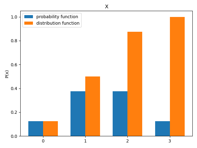
Grouped bar chart
import matplotlib.pyplot as plt
import numpy as np


labels = ['0', '1', '2', '3']
blue = [1/8, 3/8, 3/8,1/8]
orange = [1/8, 4/8, 7/8, 1]

x = np.arange(len(labels))  # the label locations
width = 0.35  # the width of the bars

fig, ax = plt.subplots()
rects1 = ax.bar(x - width/2, blue, width, label='probability function')
rects2 = ax.bar(x + width/2, orange, width, label='distribution function')

# Add some text for labels, title and custom x-axis tick labels, etc.
ax.set_ylabel('P(x)')
ax.set_title('X')
ax.set_xticks(x)
ax.set_xticklabels(labels)
ax.legend()

fig.tight_layout()

plt.show()
Histogram
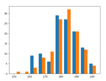
- Use plt.hist to generate a histogram of the heights of the students of classroom 1. You can use a second argument bins = n to set the amount of bins used to n. Try to find a suitable amount of bins or set bins = ‘auto’ to automatically pick the bins based on the size of the data.
import pandas as pd
import matplotlib.pyplot as plt

Height = pd.read_csv("Heights.csv", sep=";")
plt.hist(Height, bins=10)  # number of bins, not the size of the interval
# can use 'auto'
plt.show()
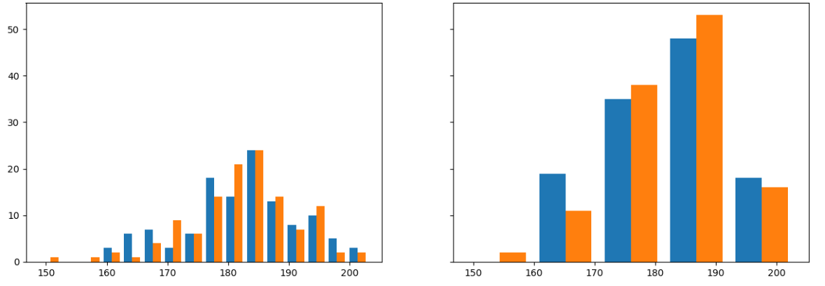
- Using the command subplots we can make multiple plots in any desired order.
- Arguments like sharex and sharey allow you to ensure that all figures have the same axes.
import pandas as pd
import matplotlib.pyplot as plt

Height = pd.read_csv("Heights.csv", sep=";")

fig, (ax1, ax2) = plt.subplots(1, 2, sharex=True, sharey=True, figsize=(15, 5))
ax1.hist(Height, bins='auto')
ax2.hist(Height, bins=5)
plt.show()
Boxplot
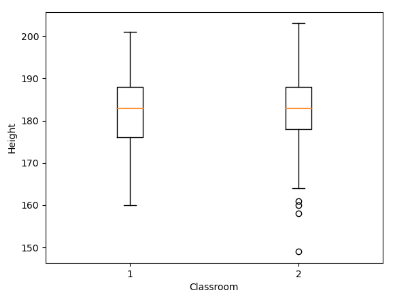
- The function plt.boxplot allows us to generate boxplots of multiple datasets next to each other if formatted correctly.
- For documentation, see https://matplotlib.org/api/_as_gen/matplotlib.pyplot.boxplot.html
import pandas as pd
import matplotlib.pyplot as plt

Height = pd.read_csv("Heights.csv", sep=";")

plt.boxplot(Height)
plt.xlabel("Classroom")
plt.ylabel("Height")
plt.show()
Numerical summaries
- from the library numpy, which is part of the library scipy that is used for most scientific operations and for all operations on arrays of data:
- .mean
- .min
- .max
- .sqrt
- .exp
- For documentation, see https://docs.scipy.org/doc/numpy/user/index.html
import pandas as pd
import numpy as np

Height = pd.read_csv("Heights.csv", sep=";")

print("The average height of Class_1 is ", np.mean(Height.Class_1))
Simulate randomness
- To get the outcome of a dice throw, we use the np.random.choice function from the library numpy.
import numpy as np

die = [1, 2, 3, 4, 5, 6]
probabilities = [1 / 6, 1 / 6, 1 / 6, 1 / 6, 1 / 6, 1 / 6]
outcome = np.random.choice(die, size=2, p=probabilities)

print("Outcome of the 2nd throw: ", outcome[1])

outcomes10 = np.random.choice(die, size=10, p=probabilities)
outcomes100 = np.random.choice(die, size=100, p=probabilities)
outcomes1000 = np.random.choice(die, size=1000, p=probabilities)

print("Average outcome after 10 throws: ", np.mean(outcomes10))
print("Average outcome after 100 throws: ", np.mean(outcomes100))
print("Average outcome after 1000 throws: ", np.mean(outcomes1000))
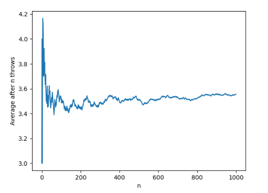
The outcome does follow the law of large numbers
import matplotlib.pyplot as plt
import numpy as np

die = [1, 2, 3, 4, 5, 6]
probabilities = [1 / 6, 1 / 6, 1 / 6, 1 / 6, 1 / 6, 1 / 6]

fig, (ax1, ax2) = plt.subplots(1, 2, sharex=True, sharey=True, figsize=(15, 5))

outcomes = np.random.choice(die, size=1000, p=probabilities)
averages = [np.mean(outcomes[range(0, i)]) for i in range(1, 1001)]

plt.plot(averages)
plt.xlabel("n")
plt.ylabel("Average after n throws")
plt.show()
Uniform distribution
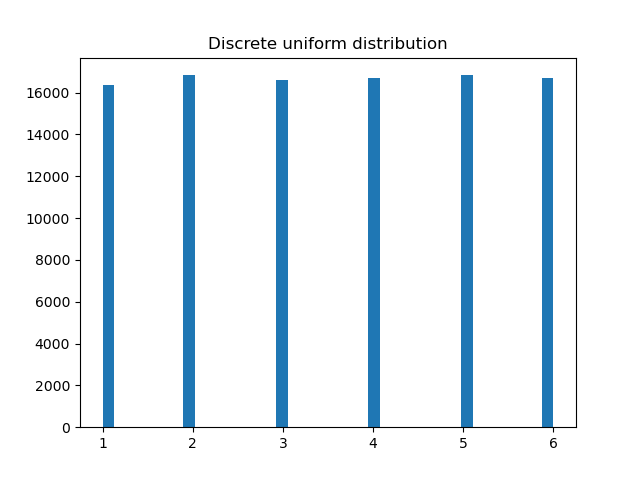
import numpy as np
import matplotlib.pyplot as plt

from scipy.stats import uniform


def die_throw_rvs(sample_size=1):
    random_variables = np.zeros(sample_size)
    uniform_variables = uniform.rvs(size=sample_size)

    random_variables = np.ceil(uniform_variables * 6)

    return random_variables


distr = die_throw_rvs(100000)
print("max: ", np.max(distr), "min: ", np.min(distr), "mean: ", np.mean(distr), "variance: ", np.var(distr))
plt.hist(distr, bins='auto')  # arguments are passed to np.histogram
plt.title("Discrete uniform distribution")

plt.show()
Discrete Gemoetric distribution
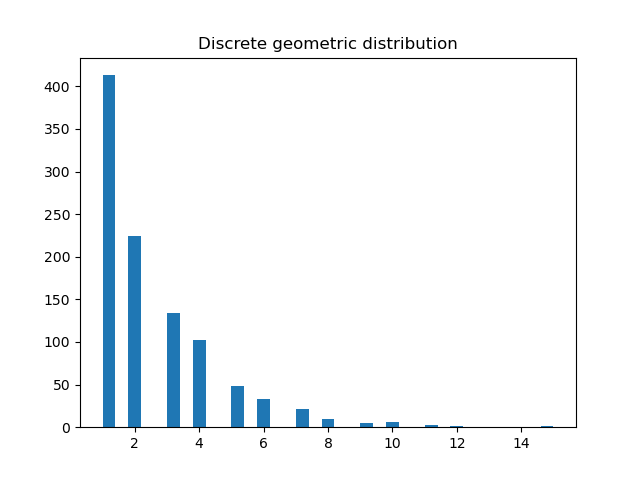
import numpy as np
import matplotlib.pyplot as plt

from scipy.stats import uniform


def die_throw_rvs(sample_size=1):
    random_variables = np.zeros(sample_size)
    uniform_variables = uniform.rvs(size=sample_size)
    random_variables = np.ceil(-1 / np.mean(uniform_variables) * np.log(uniform_variables))

    return random_variables


distr = die_throw_rvs(1000)
plt.hist(distr, bins='auto')  # arguments are passed to np.histogram
plt.title("Discrete geometric distribution")
plt.show()
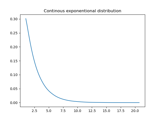
Continous Exponential distribution
import numpy as np
import matplotlib.pyplot as plt

from scipy.stats import uniform
from scipy.stats import gaussian_kde


def die_throw_rvs(sample_size=1):
    random_variables = np.zeros(sample_size)
    uniform_variables = uniform.rvs(size=sample_size)
    random_variables = -1 / np.mean(uniform_variables) * np.log(uniform_variables)

    return random_variables


distr = die_throw_rvs(100000)
density = gaussian_kde(distr)
xs = np.linspace(1, np.max(distr), 100)
density.covariance_factor = lambda: .25
density._compute_covariance()
plt.plot(xs, density(xs))
plt.title("Continous exponentional distribution")
plt.show()
